If a decision process is designed according to the expected utility (maximization) model, then the choice of an option is explained by it having the highest expected utility among considered options. Consequently, decision governance over such a decision process needs to help the decision maker predict and prepare for unexpected events in order to maximize utility.
This text is part of the series on decision governance. Decision Governance is concerned with how to improve the quality of decisions by changing the context, process, data, and tools (including AI) used to make decisions. Understanding decision governance empowers decision makers and decision stakeholders to improve how they make decisions with others. Start with “What is Decision Governance?” and find all texts on decision governance here.
What is the topic of this text?
If a decision process is designed according to the expected utility model, then, one, How does it explain decisions? two, How to influence that process through governance?, and three, How is this different from governing a decision process modeled after classical utility maximization?
Why is this topic relevant for decision governance?
The expected utility maximization model, or simply the expected utility model (see Briggs, 2023 for an overview of key ideas) is the simplest decision making model in which options have uncertain outcomes.
This is also the simplest model to use, to look at how decision governance can handle uncertainty of options.
Background: What is the expected utility (maximization) model?
In the expected utility model, we have the following:
- One decision maker
- Options that the decision maker chooses from
- Alternative future states that influence the outcome of decisions
- The probability that each future state occurs, with the sum of the probabilities of all considered future states being equal to 1
- For each option, its utility in each future state
- The assumption that the decision maker will choose the option which will lead to the highest total utility over all considered future states
We assume that the decision is made as follows:
- A decision maker identifies options.
- The decision maker predicts future states for each option.
- The decision maker assigns a probability to each future state of an option, such that the sum of probabilities over all future states for an option is equal to 1.
- The decision maker assigns a utility to each option in each of its considered future states.
- The decision maker calculates the expected utility of each option, by summing the product of that option’s utility in each of its future states, weighted by the probability of the future state.
Example: Decision making with the expected utility model
Consider the following example.
In The Iliad by Homer, Achilles, the Greek hero, decides to withdraw from battle after a dispute with Agamemnon, the leader of the Greek forces during the Trojan War. Agamemnon, having been forced to return his war prize, Chryseis, to appease the gods, demands Achilles’ prize, Briseis, as compensation. In response, Achilles, feeling dishonored and enraged by Agamemnon’s actions, chooses to withdraw himself and his troops from the fighting, despite the consequences for the Greek army.
Let’s make up some hypothetical probability and utility values for Achilles, and see how the model would explain his decision.
- Identifying Options: Achilles has two options:
- Option 1: Remain in battle.
- Option 2: Withdraw from battle.
- Predicting Future States: For each option, Achilles considers two possible future states:
- Future States for Option 1 (Remain in battle):
- State 1.1: The Greek forces win the war, but Achilles feels dishonored. Probability: p_1.1 = 0.6.
- State 1.2: The Greek forces lose the battle despite his efforts, but Achilles’ honor remains tarnished. Probability: p_1.2 = 0.4.
- Future States for Option 2 (Withdraw from battle):
- State 2.1: The Greek forces struggle and suffer significant losses without Achilles’ support, but Agamemnon’s leadership is questioned. Probability: p_2.1 = 0.7.
- State 2.2: The Greek forces adapt and eventually find a way to win without Achilles, and his honor remains intact. Probability: p_2.2 = 0.3.
- Future States for Option 1 (Remain in battle):
- Assigning Utilities to Each Option in Each Future State: Achilles assigns utility values to each outcome based on how much he values each future scenario.
- Utilities for Option 1 (Remain in battle):
- Utility of State 1.1: U(1.1) = 30 (value of Greek victory with dishonor).
- Utility of State 1.2: U(1.2) = 10 (value of Greek loss with dishonor).
- Utilities for Option 2 (Withdraw from battle):
- Utility of State 2.1: U(2.1) = 50 (value of Greek struggle with Agamemnon’s leadership questioned).
- Utility of State 2.2: U(2.2) = 40 (value of Greek victory without dishonor).
- Utilities for Option 1 (Remain in battle):
- Calculating the Expected Utility of Each Option:
- Expected Utility of Option 1 (Remain in battle):
- EU(1) = (p_1.1 * U(1.1)) + (p_1.2 * U(1.2))
- EU(1) = (0.6 * 30) + (0.4 * 10)
- EU(1) = 18 + 4 = 22
- Expected Utility of Option 2 (Withdraw from battle):
- EU(2) = (p_2.1 * U(2.1)) + (p_2.2 * U(2.2))
- EU(2) = (0.7 * 50) + (0.3 * 40)
- EU(2) = 35 + 12 = 47
- Expected Utility of Option 1 (Remain in battle):
- Decision: Based on the above, the expected utility of remaining in battle is 22, while the expected utility of withdrawing from battle is 47. According to the expected utility model, Achilles would choose to withdraw from the battle because it maximizes his expected utility.
What is the explanation of a decision in this decision model?
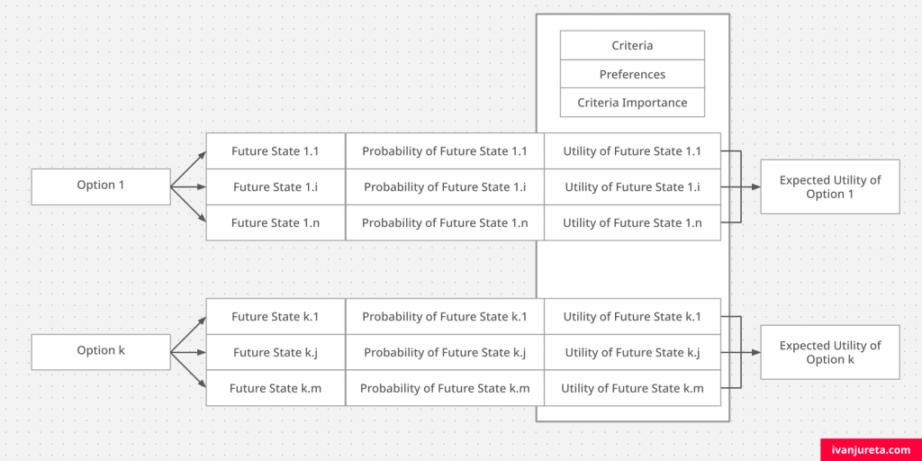
Explanation of a decision in the expected utility model is more complicated than in the classical utility maximization one (see the text here). While criteria, preferences, and criteria importance are still there, as there would otherwise be no utility, uncertainty makes information about options more complicated.
The choice of an option depends on future states of options, their utility and uncertainty associated with them. Probability is simply a measure of uncertainty. The figure below shows this complication. The reason why, say Option 1 is chosen, is that it has highest expected utility – which simply leads to the questions about which preferences, criteria and criteria importance were considered, but also which future states we predicted of that option, and the uncertainty we assumed they have.
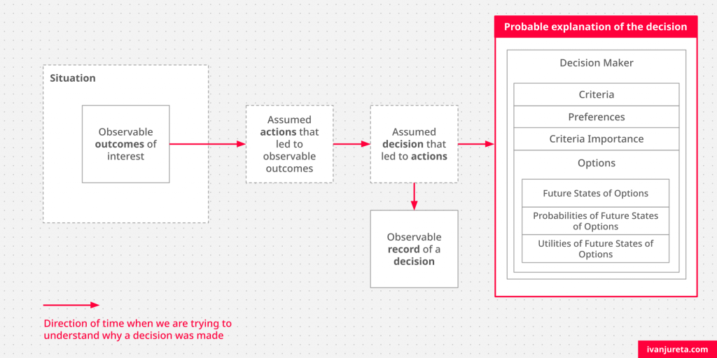
The next figure, below, shows the same elements in the same diagram I used in previous texts, for other decision models.
How to influence this decision process through governance?
I discussed in the text on the classical utility maximization model, here, some common ways to influence options which are considered, as well as preferences and criteria. To influence prediction of future states and the evaluation of their uncertainty, typical types of strategies include the following.
- Data and Analytics: We can require that data is collected and analyzed in specific ways ahead of decision making, both before options are defined, or when they are known.
- Training and Experience: Training in decision analysis methods such as scenario planning and decision trees can be helpful when thinking through potential future states and their probability. Domain expertise plays a critical role.
- Bias Reduction: Debiasing strategies and nudges help mitigate cognitive distortions like overconfidence and anchoring, improving probability assessments.
- Expert and Group Input: Methods like the Delphi technique and structured group discussions reinforce the importance of gathering information from others.
- Scenario Planning and Stress Testing: Scenario planning encourages a broader view of possible outcomes, while stress testing evaluates decision performance under less likely conditions.
References and Further Reading
- Briggs, R. A., “Normative Theories of Rational Choice: Expected Utility”, The Stanford Encyclopedia of Philosophy (Winter 2023 Edition), Edward N. Zalta & Uri Nodelman (eds.), URL = <https://plato.stanford.edu/archives/win2023/entries/rationality-normative-utility/>.
- Gelman, A., et al. (2013). Bayesian Data Analysis. CRC Press.
- Linstone, H. A., & Turoff, M. (1975). The Delphi Method: Techniques and Applications. Addison-Wesley.
- Tversky, Amos, and Daniel Kahneman. “Judgment under Uncertainty: Heuristics and Biases: Biases in judgments reveal some heuristics of thinking under uncertainty.” Science 185.4157 (1974): 1124-1131.
Decision Governance
This text is part of the series on the design of decision governance. Other texts on the same topic are linked below. This list expands as I add more texts on decision governance.
- Introduction to Decision Governance
- Stakeholders of Decision Governance
- Foundations of Decision Governance
- How to Spot Decisions in the Wild?
- When Is It Useful to Reify Decisions?
- Decision Governance Is Interdisciplinary
- Individual Decision-Making: Common Models in Economics
- Group Decision-Making: Common Models in Economics
- Individual Decision-Making: Common Models in Psychology
- Group Decision-Making: Common Models in Organizational Theory
- Role of Explanations in the Design of Decision Governance
- Design of Decision Governance
- Design Parameters of Decision Governance
- Factors influencing how an individual selects and processes information in a decision situation, including which information the individual seeks and selects to use:
- Psychological factors, which are determined by the individual, including their reaction to other factors:
- Attention:
- Memory:
- Mood:
- Emotions:
- Commitment:
- Temporal Distance:
- Social Distance:
- Expectations
- Uncertainty
- Attitude:
- Values:
- Goals:
- Preferences:
- Competence
- Social factors, which are determined by relationships with others:
- Impressions of Others:
- Reputation:
- Promises:
- Social Hierarchies:
- Social Hierarchies: Why They Matter for Decision Governance
- Social Hierarchies: Benefits and Limitations in Decision Processes
- Social Hierarchies: How They Form and Change
- Power: Influence on Decision Making and Its Risks
- Power: Relationship to Psychological Factors in Decision Making
- Power: Sources of Legitimacy and Implications for Decision Authority
- Power: Stability and Destabilization of Legitimacy
- Power: What If High Decision Authority Is Combined With Low Power
- Power: How Can Low Power Decision Makers Be Credible?
- Social Learning:
- Psychological factors, which are determined by the individual, including their reaction to other factors:
- Factors influencing information the individual can gain access to in a decision situation, and the perception of possible actions the individual can take, and how they can perform these actions:
- Governance factors, which are rules applicable in the given decision situation:
- Incentives:
- Incentives: Components of Incentive Mechanisms
- Incentives: Example of a Common Incentive Mechanism
- Incentives: Building Out An Incentive Mechanism From Scratch
- Incentives: Negative Consequences of Incentive Mechanisms
- Crowding-Out Effect: The Wrong Incentives Erode the Right Motives
- Crowding-In Effect: The Right Incentives Amplify the Right Motives
- Rules
- Rules-in-use
- Rules-in-form
- Institutions
- Incentives:
- Technological factors, or tools which influence how information is represented and accessed, among others, and how communication can be done
- Environmental factors, or the physical environment, humans and other organisms that the individual must and can interact with
- Governance factors, which are rules applicable in the given decision situation:
- Factors influencing how an individual selects and processes information in a decision situation, including which information the individual seeks and selects to use:
- Change of Decision Governance
- Public Policy and Decision Governance:
- Compliance to Policies:
- Transformation of Decision Governance
- Mechanisms for the Change of Decision Governance